library("tidyverse")
library("ggdensity")
library("ggridges")
library("Lahman")
library("DT")Moneyball in R
A Quick and Incomplete Introduction
Welcome to Opening Day 2023! This post will serve as a (very quick and incomplete) introduction to “Moneyball” using R. For students in STAT 385, it will help reinforce various concepts from the tidyverse.
To set the stage, we recommend the following video:
Setup
# install.packages("remotes")
remotes::install_github("daviddalpiaz/bbd")
All-Time Homerun Leaders
Batting |>
  select(playerID, yearID, teamID, HR) |>
  summarise(HR = sum(HR), .by = playerID) |>
  filter(HR >= 100) |>
  arrange(desc(HR)) |>
  left_join(People, by = "playerID") |>
  select(playerID, nameFirst, nameLast, HR) |>
  unite(Name, nameFirst:nameLast, sep = " ") |>
  left_join(
    summarise(HallOfFame, inHall = "Y" %in% inducted, .by = playerID),
    by = "playerID"
  ) |>
  datatable()
Pythagorean Theorem of Baseball
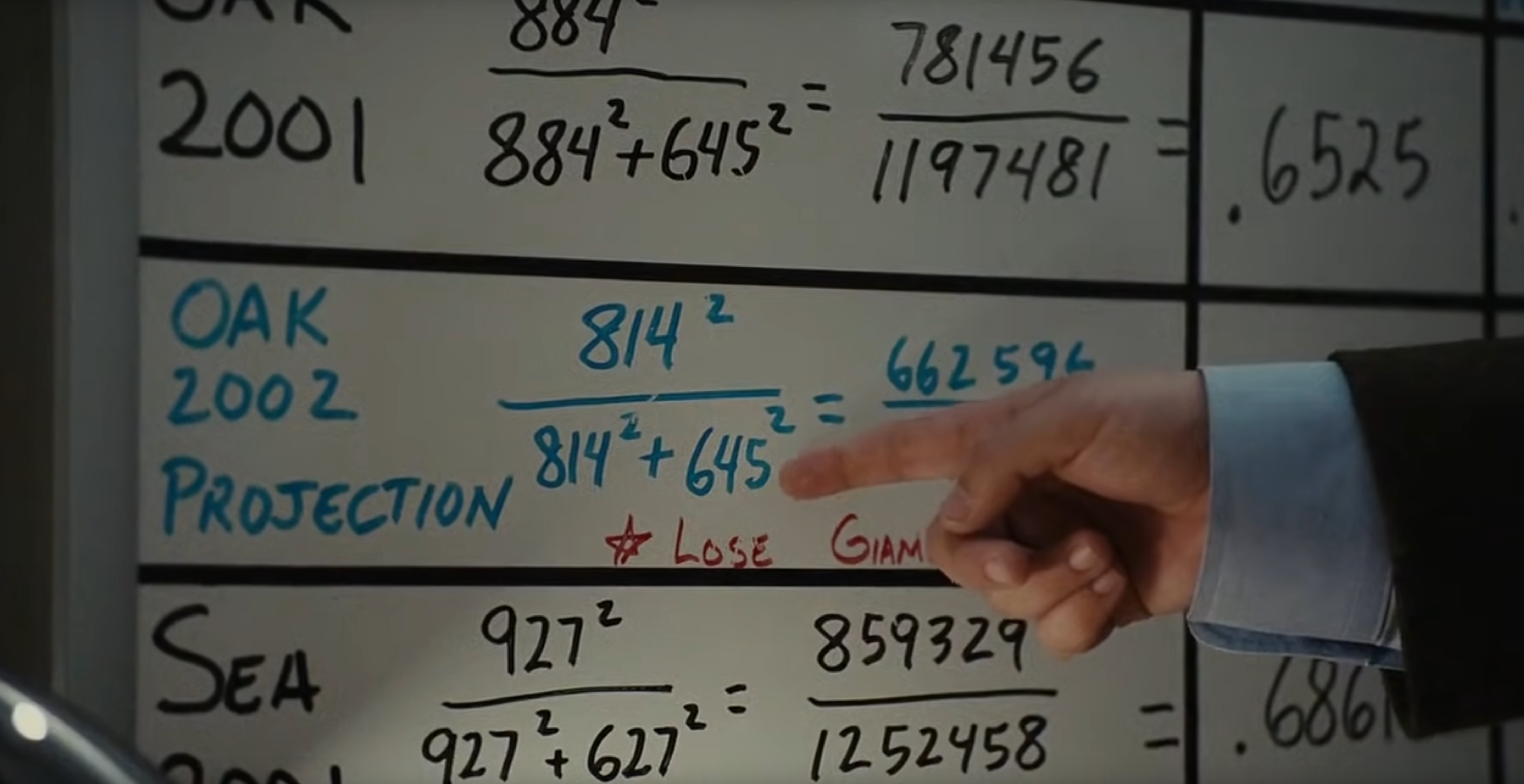
Teams |>
  select(yearID, teamID, W, L, R, RA) |>
  arrange(desc(yearID)) |>
  filter(yearID > 1990) |>
  mutate(pythWPerc = (R ^ 2) / (R ^ 2 + RA ^ 2)) |>
  mutate(pythW = round(pythWPerc * 162)) |>
  mutate(weirdSeason = case_when(
    yearID == 2020 ~ "2020, COVID",
    yearID == 1994 ~ "1994, Strike",
    .default = "Normal")
  ) |>
  ggplot() +
  aes(x = W, y = pythW, color = weirdSeason) +
  geom_point() +
  geom_smooth(method = "lm") +
  scale_color_brewer(palette = "Set1") +
  theme_bw()
`geom_smooth()` using formula = 'y ~ x'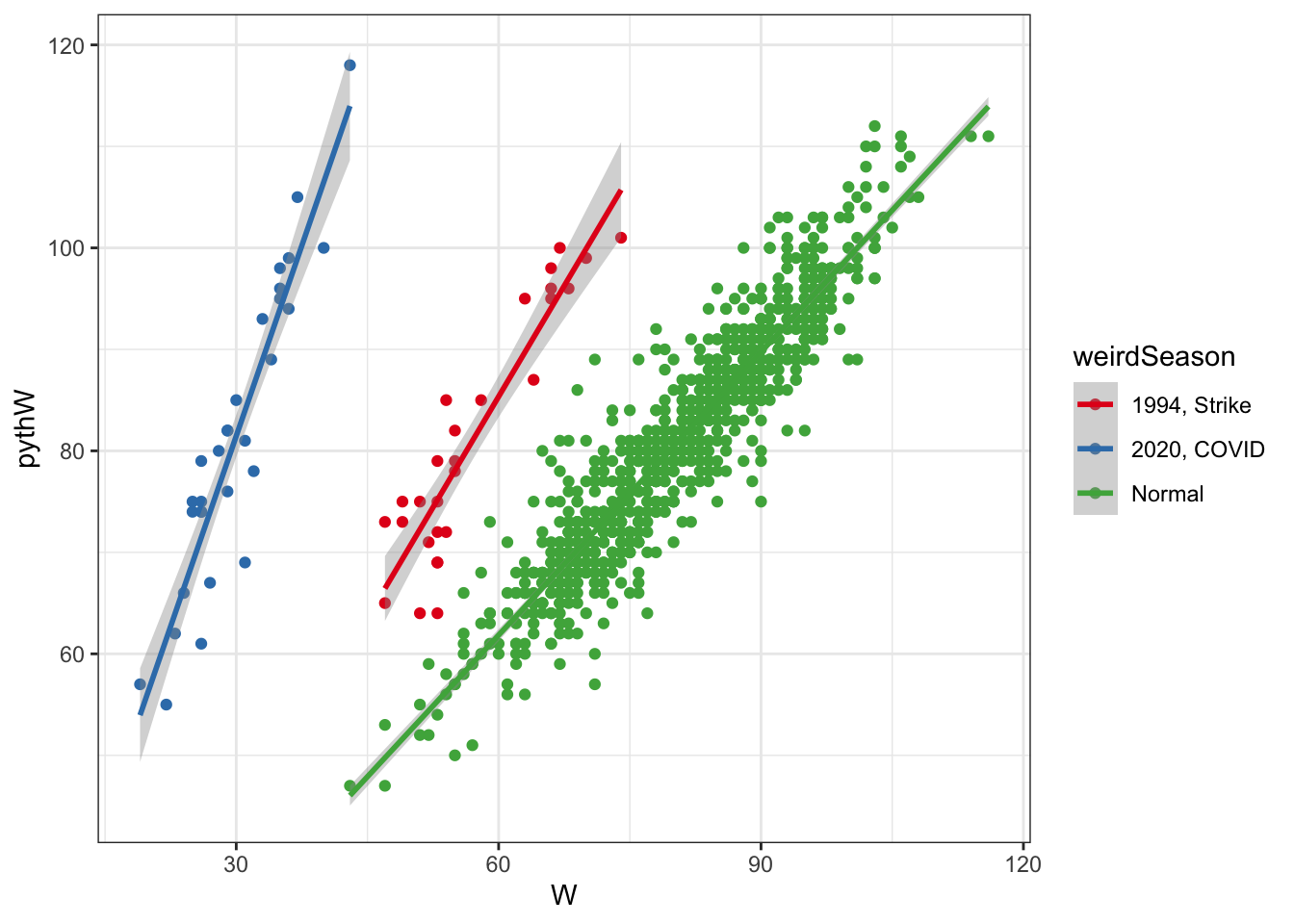
- TODO: do only 2021
- TODO: multiply by games instead of 162
Pitching Metrics
- https://baseballsavant.mlb.com/
- https://baseballsavant.mlb.com/savant-player/dylan-cease-656302?stats=statcast-r-pitching-mlb
- https://baseballsavant.mlb.com/csv-docs
- https://daviddalpiaz.github.io/bbd/
bbd::people_search("Dylan Cease")# A tibble: 6 × 5
name birth_year key_mlbam key_bbref key_fangraphs
<chr> <int> <int> <chr> <int>
1 Dylan Chavez 1991 605178 "" NA
2 Dylan Castaneda 2001 688341 "" NA
3 Dylan Neuse 1998 681540 "" NA
4 Dylan Cease 1995 656302 "ceasedy01" 18525
5 Dylan Beavers 2001 687637 "" NA
6 Dylan Beasley 1997 670188 "" NAsc2022 = bbd::statcast_bbd(start = "2022-01-01", end = "2022-12-13", verbose = TRUE)
cease2022 = filter(sc2022, pitcher == 656302)
saveRDS(cease2022, file = "data/cease2022.rds")cease2022 = readRDS("data/cease2022.rds")geom_strikezone = function(color = "black", linewidth = 0.25, sz_top = 3.8, sz_bot = 1.1) {
sz_left = -0.85
sz_right = 0.85
strikezone = data.frame(
x = c(sz_left, sz_left, sz_right, sz_right, sz_left),
y = c(sz_bot, sz_top, sz_top, sz_bot, sz_bot)
)
geom_path(aes(.data$x, .data$y), data = strikezone, linewidth = linewidth, col = color)
}cease2022 |>
filter(stand == "R") |>
filter(!is.na(pitch_type)) |>
ggplot() +
aes(x = plate_x, y = plate_z) +
geom_hdr(
method = method_kde(),
probs = c(0.95, 0.75, 0.50, 0.25, 0.05)
) +
geom_strikezone() +
geom_point(
aes(color = pitch_type),
alpha = 0.4
) +
theme_bw() +
theme(
aspect.ratio = 1,
legend.position = c(1, 0),
legend.justification = c(1, 0),
legend.box = "horizontal"
) +
scale_color_brewer(palette = "Set1") +
facet_wrap(vars(pitch_type))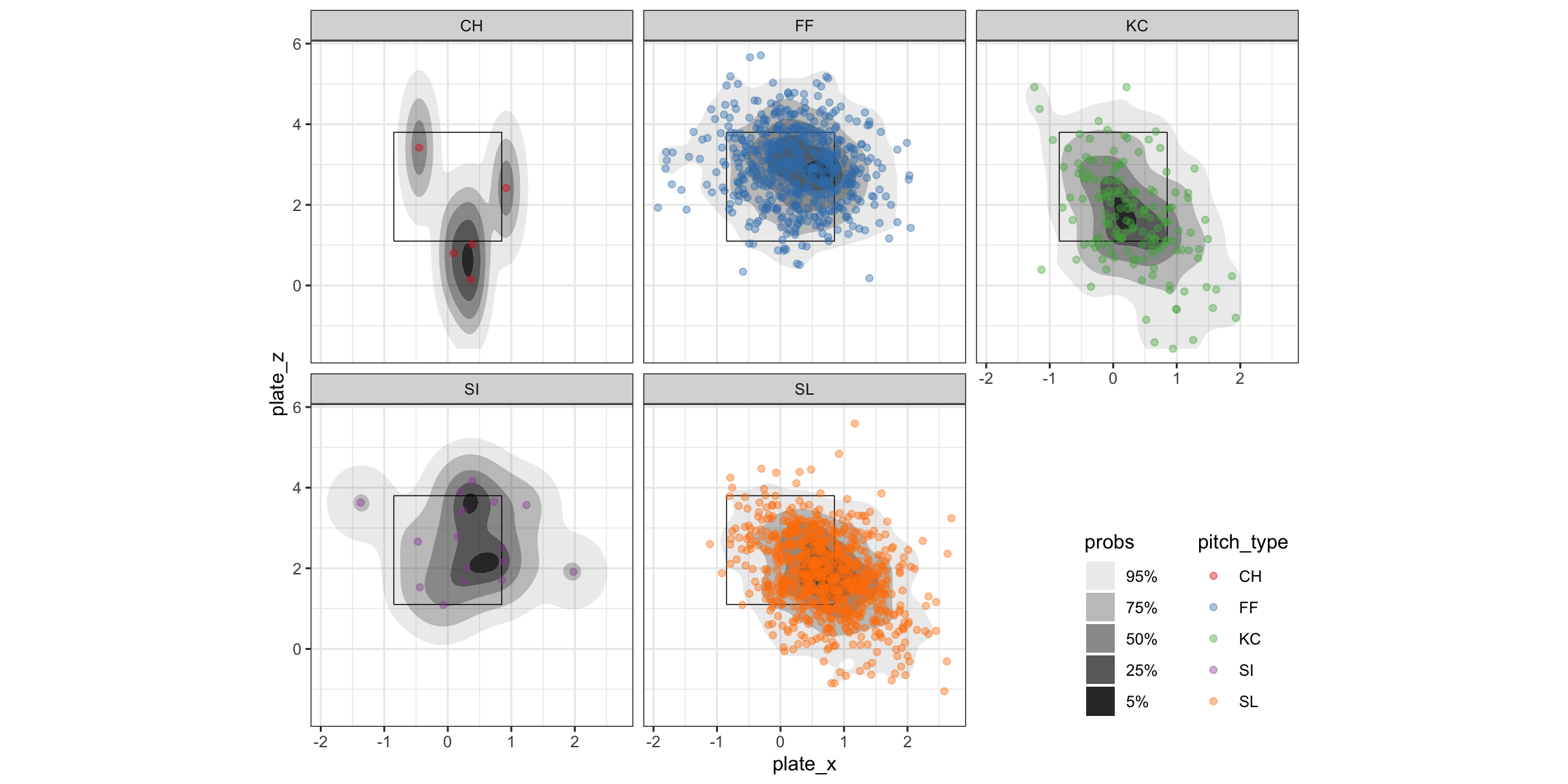
cease2022 |>
  filter(!is.na(pitch_type)) |>
  ggplot() +
  aes(x = release_speed, y = pitch_type, fill = pitch_type) +
  geom_density_ridges() +
  scale_fill_brewer(palette = "Set1") +
  theme_bw()
Picking joint bandwidth of 0.472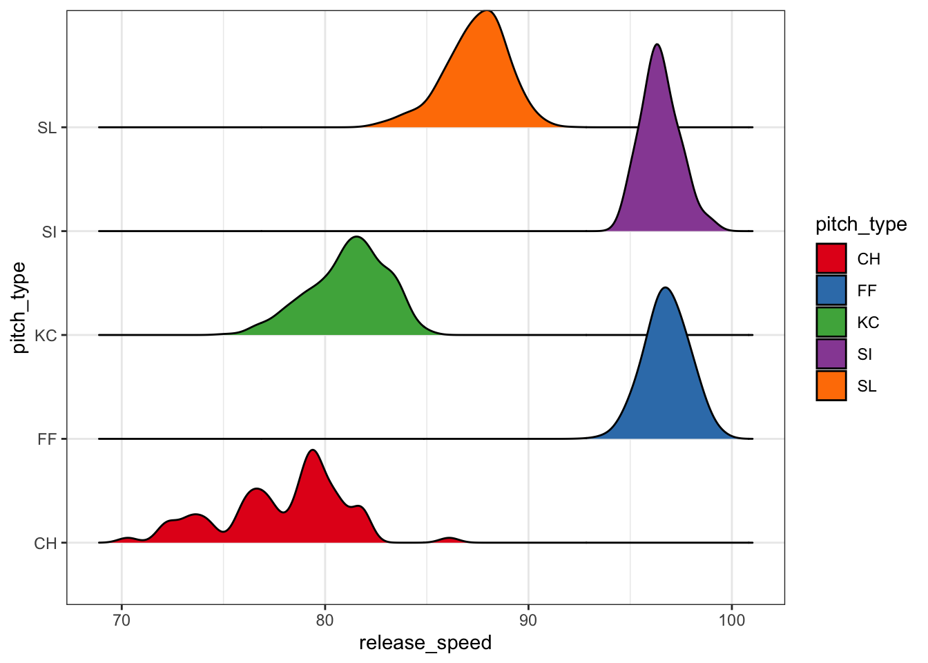
cease2022 |>
  filter(!is.na(pitch_type)) |>
  ggplot() +
  aes(x = release_speed, y = release_spin_rate) +
  geom_point(aes(color = pitch_type), alpha = 0.4, size = 2) +
  theme_bw() +
  scale_color_brewer(palette = "Set1")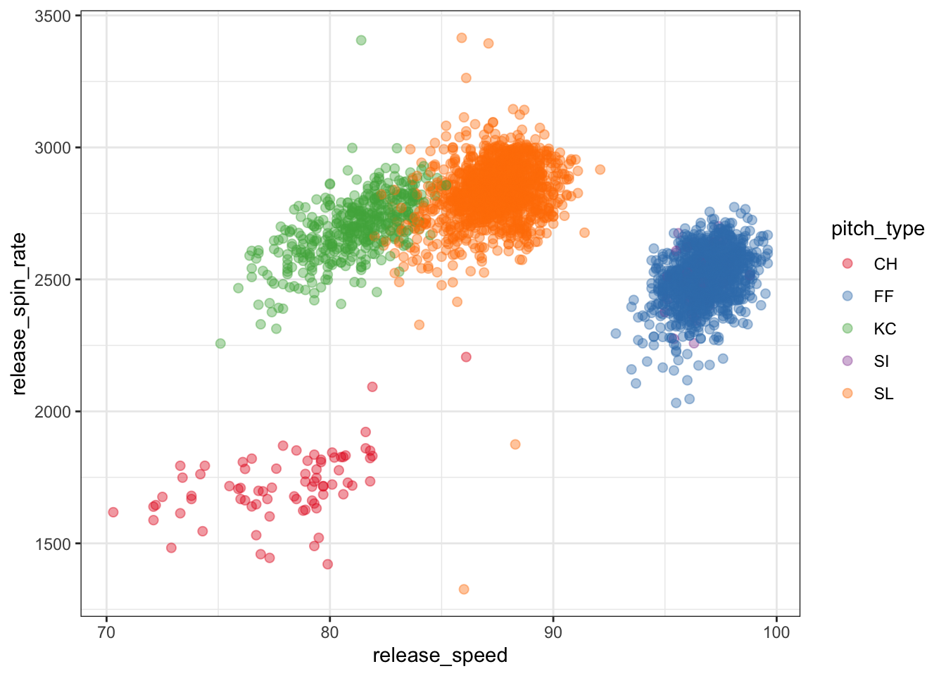
cease2022 |>
  filter(!is.na(pitch_type)) |>
  summarise(
    n = n(),
    velo = round(mean(release_speed), digits = 1),
    spin = round(mean(release_spin_rate), digits = 1),
    h_move = round(mean(pfx_x), digits = 2),
    v_move = round(mean(pfx_z), digits = 2),
    .by = c(pitch_type, pitch_name)) |>
  arrange(desc(n)) |>
  datatable(
    rownames = FALSE,
    options = list(dom = 't'),
    colnames = c(
      "Pitch Type" = "pitch_type",
      "Pitch Name" = "pitch_name",
      "Number Thrown" = "n",
      "Average Velocity" = "velo",
      "Average Spin" = "spin",
      "Average Horizontal Movement" = "h_move",
      "Average Vertical Movement" = "v_move"
    )
  )
Baseball Analytics at Illinois
- Eck Lab
- https://baseball.physics.illinois.edu/
- https://stat.illinois.edu/news/2023-03-13/statistics-and-story-baseballs-two-languages
- https://stat.illinois.edu/news/2022-12-19/new-statistics-course-takes-swing-baseball-analytics
- https://stat.illinois.edu/news/2021-11-30/illinois-alumnus-steps-bat-chicago-cubs-new-assistant-general-manager
- https://stat.illinois.edu/news/2020-05-14/deck-charlie-young-statistics-major-heads-major-leagues